TUTORIAL 5 - Excel Review

This tutorial is designed to be a refresher for all of the concepts that you will want to have some experience with before moving on to the following tutorials. It’s purpose is to kick off an Excel unit in a higher level comptuer applications class.

Here’s the list of skills we want to cover:

 Cells, Rows, Columns
 Table Formatting (and its uses
 Basic Formulas and Functions
 Fill Handle
 Basic Charts

Tutorial

Download the start file.

Basic Editing

First, we are going to look at the basic editing techniques. We will assume basic familiarity with the interface (what a cell is, etc).

On the documentation sheet, click the link for the first exercise.

1. For Exeercise 1, select cells B6:B7. Click on the fill handle

   

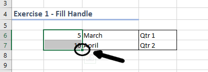
   and drag the mouse down two cells, so your screen looks like this:

   

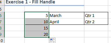
   Notice that Excel follows the same pattern established in the first two cells. Do the same with the cells C6:C7 and D6:D7

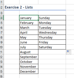
2. Next, use the fill handle to fill in the names of the months and days of the week in Exercise 2:

   

3. In Exercise 3, select cell F30. Enter the formula =SUM(C30:E30). Alternately, the Autosum tool should work:

   

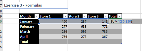
   When you press enter, notice that it fills in the rest of the column. Next, select cell C35 and type =SUM(. Next, use the mouse to select cells C30:C33. Press Enter. Finally, use the fill handle to fill in cells D34:E34.

4. For the final exercise on this sheet, most of the formulas are already generated. But you will have to do some detail. Select cells E41:G41. Drag the fill handle down to fill in the table:

   

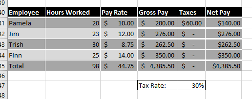
   Notice that the taxes column is all wrong, and hence, the Net Pay column is all wrong as well. THe reason for this is that it uses a relative reference get the Tax Rate from cell F47. To fix this, select cell F41. Then, edit the formula so that it reads =E41*$F$47. Press Enter and then drag the fill handle down to correct the entire table.

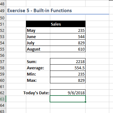
5. In cell C57, enter the formula for the SUM function. Your goal is to add the sales numbers from the above table. Thus, your fomula should look like this: =SUM(C52:C55). Do the same for the next three cells. In C58:C60, add the formulas for AVERAGE, MIN, and MAX respectively. It should look like this:

   

Charting

On the next sheet, we’ll build a few charts.

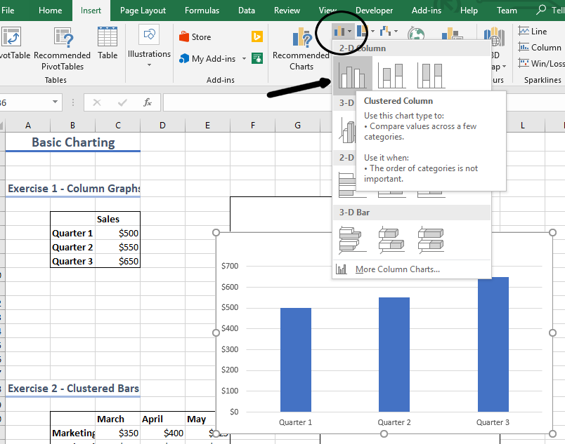
1. First, select the entire box of data, that is, cells B6:C9. In the Insert tab, click the Clustered Column. Choose the first one and style it however you like.

   

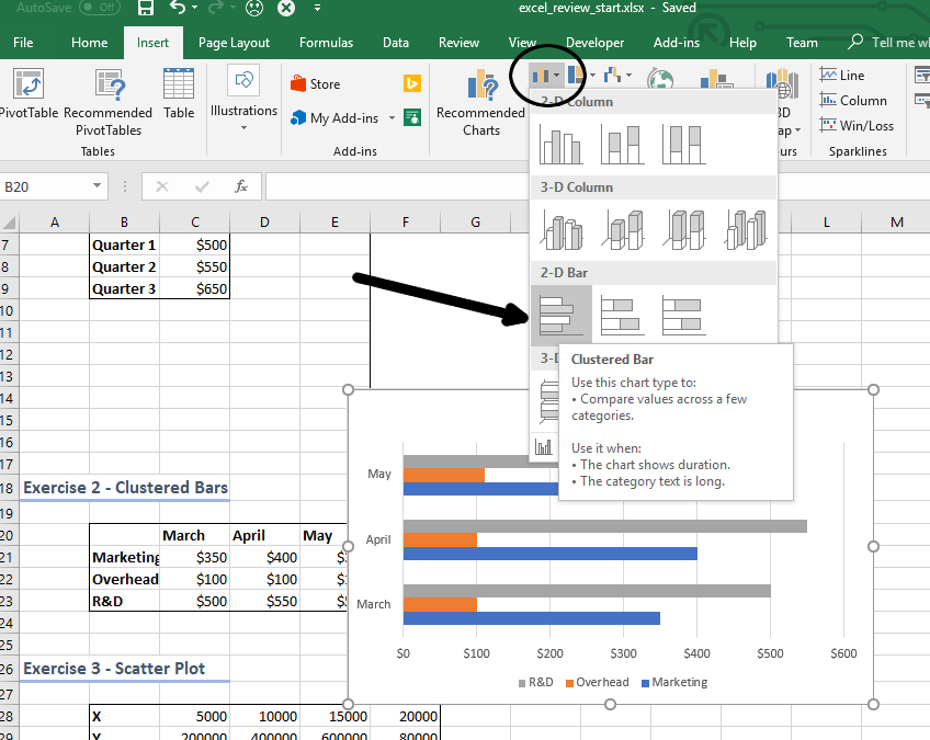
2. Next, select the cells B20:E23. Click the Clustered Column tool again, but this time use the Clustered Bar graph.

   

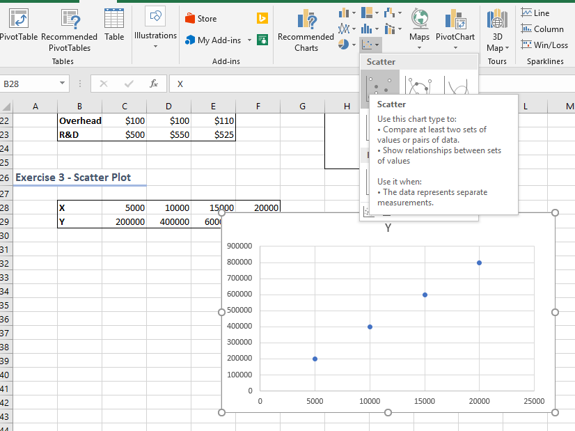
3. Finally, select cells B28:F29. Choose the Scatter Plot as shown in the following screenshot.

   

4. Challenge: Create a pie chart from the labels and the totals from the Cookie Sales table. You will have to generate the totals yourself.

Conclusion

When you are finished, upload the resulting file to the course portal as normal.

---